wingolog

Greets, and welcome back to the solipsism! I've been wandering the wilderness with my Guile hackings lately, but I'm finally ready to come back to civilization. Hopefully you will enjoy my harvest of forest fruit.

Today's article is about flow analysis and data structures. Ready? Let's rock!

flow analysis

Many things that a compiler would like to know can be phrased as a question of the form, "What do I know about the data flowing through this particular program point?" Some things you might want to know are:

1. The set of variables that must be live.

2. The set of variables that happen to be live. This is the same as (1) except it includes variables that aren't needed but haven't been clobbered by anything.

3. The set of expressions whose results are still valid (i.e., haven't been clobbered by anything else).

4. An upper and lower bound on the range of numeric variables.

Et cetera. I'll talk about specific instances of flow analysis problems in the future, but today's article is a bit more general.

The first thing to note about these questions is that they don't necessarily need or have unique answers. If GCC decides that it can't prove anything about the ranges of integers in your program, it's not the end of the world -- it just won't be able to do some optimizations that it would like to do.

At the same time, there are answers that are better and worse than others, and answers that are just invalid. Consider a function of the form:

int f():
  int a = 1
  int b = 2
  int c = a + b
  int d = b + c
  ...
  int z = x + y
  return z

In this function, there are 27 different expressions, including the return, and 27 different program points. (You can think of a program point as a labelled sub-expression. In this example none of the expressions have sub-expressions.) If we number the program points in order from 0 to 26, we will have a program that first executes expression 0 (int a = 1), then 1, and so on to the end.

Let's plot some possible solutions to the live variable flow-analysis problem for this program.

Here we see two solutions to the problem (in light and dark blue), along with a space of invalid solutions (in red). The Y axis corresponds to the variables of the program, starting with a on the bottom and finishing with z on the top.

For example, consider position 4 in the program, corresponding to int e = c + d. It is marked in the graph with a vertical bar. After position 4, the only values that are used in the rest of the program are d and e. These are the variables that are contained within the light-blue area. It wouldn't be invalid to consider a, b, and c to be live also, but it also wouldn't be as efficient to allocate space and reason about values that won't contribute to the answer. The dark blue space holds those values that may harmlessly be considered to be live, but which actually aren't live.

It would, however, be invalid to consider the variable f to be live after position 4, because it hasn't been defined yet. This area of the variable space is represented in red on the graph.

Of course, the space of all possible solutions isn't possible to represent nicely on a two-dimensional graph; we're only able to show two with colors, and that not very well as they overlap. This difficulty cuts close to the heart of the data-flow problem: that it ultimately requires computing a two-dimensional answer, which necessarily takes time and space O(n²) in program size.

Or does it?

classical flow analysis frameworks

The classical way to do flow analysis is to iterate a set of data-flow equations over an finite lattice until you reach a fixed point.

That's a pithy sentence that deserves some unpacking. If you're already comfortable with what it means, you can skip a couple sections.

Still here? Cool, me too. Let's take a simple example of sign analysis. The problem is to determine, for the integer variables of a program, at every point in the program, which ones may be negative (-), which ones may be zero (0), and which may be positive (+). All of these are conceptually bit-flags.

For example, in this program:

int f(int x):
 L0:  while (x >= 0)
 L1:    int y = x - 1
 L2:    x = y
 L3:  return x

We can assign the flags -0+ to the argument x as the initial state that flows into L0, because we don't know what it is ahead of time, and it is the only variable in scope. We start by representing the initial state of the solution as a set of sets of state values:

state := {L0: {x: -0+}, L1: Ø, L2: Ø, L3: Ø}

In this notation, Ø indicates a program point that hasn't been visited yet.

Now we iterate through all labels in the program, propagating state to their successors. Here is where the specific problem being solved "hooks in" to the generic classical flow analysis framework: before propagating to a successor, a flow equation transforms the state that flows into a program point to a state that flows out, to the particular successor. In this case we could imagine equations like this:

visit_test(expr, in, true_successor, false_successor):
  if expr matches "if var >= 0":
    # On the true branch, var is not negative.
    propagate(in + {var: in[var] - -}, true_successor)
    # On the false branch, var is not zero and not positive.
    propagate(in + {var: in[var] - 0+}, false_successor)
  else if ...

visit_expr(expr, in, successor):
  if expr matches "left = right - 1":
    if in[right] has +:
      if in[right] has 0:
        # Subtracting one from a non-negative arg may be negative.
        propagate(in + {left: in[right] + -}, successor)
      else
        # Subtracting one from a positive arg may be 0.
        propagate(in + {left: in[right] + 0}, successor)
    else:
      # Subtracting one from a nonpositive arg will be negative.
      propagate(in + {left: -}, successor)
  else if expr matches "left = right":
    propagate(in + {left: in[right]}, successor)
  ...

The meat of classical data-flow analysis is the meet operation:

propagate(out, successor):
  if state[successor] is Ø:
    state[successor] = out
  else
    state[successor] = meet(out, state[successor]):

# A version of meet for sign analysis
meet(out, in):
  return intersect_vars_and_union_values(out, in)

Let's run this algorithm by hand over the example program. Starting from the initial state, we propagate the L0→L1 and L0→L3 edges:

visit_test("if x <= 0", {x: -0+}, L1, L3)
→ propagate({x: 0+}, L1)
→ state[L1] = {x: 0+}
→ propagate({x: -}, L3)
→ state[L3] = {x: -}

Neat. Let's keep going. The successor of L1 is L2:

visit_expr("y = x - 1", {x: 0+}, L2)
→ propagate({x: 0+, y: -0+}, L2)
→ state[L2] = {x: 0+, y: -0+}

L2→L0 is a back-edge, returning to the top of the loop:

visit_expr("x = y", {x: 0+, y: -0+}, L0)
→ propagate({x: -0+, y: -0+}, L0)
→ state[L0] = meet({x: -0+, y: -0+}, state[L0])
→ state[L0] = meet({x: -0+, y: -0+}, {x: -0+})
→ state[L0] = {x: 0+}

Finally, L3 has no successors, so we're done with this iteration. The final state is:

{L0: {x: -0+},
 L1: {x: 0+},
 L2: {x: 0+, y: -0+},
 L3: {x: -}}

which indeed corresponds with what we would know intuitively.

fixed points and lattices

Each of the steps in our example flow analysis was deterministic: the result was calculated from the inputs and nothing else. However the backwards branch in the loop, L2→L0, could have changed inputs that were used by the previous L0→L1 and L0→L3 forward edges. So what we really should do is iterate the calculation to a fixed point: start it over again, and run it until the state doesn't change any more.

It's easy to see in this case that running it again won't end up modifying the state. But do we know that in all cases? How do we know that iteration would terminate at all? It turns out that a few simple conditions are sufficient.

The first thing to ensure is that state space being explored is finite. Here we can see this is the case, because there are only so many ways you can combine -, 0, and +. Each one may be present or not, and so we have 2ⁿ = 2³ = 8 possible states. The elements of the state array will be a set with at most one entry for each variable, so the whole state space is finite. That at least ensures that an answer exists.

Next, the "meet" operation has to be commutative, associative, and idempotent. The above example used intersect_vars_and_union_values. We intersect vars because it only makes sense to talk about a variable at a program point if the variable dominates the program point. It didn't make sense to propagate y on the L2→L0 branch, for example. It's usually a good idea to model a data-flow problem using sets, as set union and intersection operations fulfill these commutative, associative, and distributive requirements.

Finally, the state being modelled should have a partial order, and functions that add information along control-flow edges -- above, visit_test and visit_expr -- should preserve this partial ordering. That is to say, visit_test and visit_expr should be monotonic. This means that no matter on what control paths data propagates, we keep building towards an answer with more information, making forward progress. This condition is also easily fulfilled with sets, or more generally with any lattice. (A lattice is nothing more than a data type that fulfills these conditions.)

Iterating the data-flow equations until the state stops changing will find a fixed point of the lattice. Whether you find the greatest or least fixed point is another question; I can't help linking to Paul Khuong's old article on Québécois student union strikes for a lovely discussion.

Another question is, how many iterations are necessary to reach a fixed point? I would first note that although in our walk-through we iterated in forward order (L0, L1, L2, L3), we could have visited nodes in any order and the answer would be the same. I'll cut to the chase and say that if:

1. you represent your state with bitvectors

2. the control-flow graph is reducible (has only natural loops)

3. the meet operation on values is bitvector union or intersection

4. you visit the program points in topologically sorted order

If these conditions are fulfilled, then you will reach a fixed point after LC + 2 iterations, where LC is the "loop-connectness number" of your graph. You can ensure (1), (3), and (4) by construction. (Reverse post-order numbering is an easy way to fulfill (4).) (2) can be ensured by using programming languages without goto (a for loop is always a natural loop) but can be violated by optimizing compilers (for example, via contification).

Loop connectedness is roughly equivalent to the maximum nesting level of loops in the program, which has experimentally been determined to rarely exceed 3. Therefore in practice, data-flow analysis requires a number of steps that is O(n * 5) = O(n) in program size.

For more information on data-flow analysis, including full proofs and references, see Carl Offner's excellent, excellent manuscript "Notes on Graph Algorithms used in Optimizing Compilers". I don't know of any better free resource than that. Thanks, Carl!

an aside: the kCFA algorithms

I just finished describing what I called "classical" data-flow analysis. By that I mean to say that people have been doing it since the 1970s, which is classical enough as far as our industry goes. However with the rise of functional languages in the 1980s, it became unclear how to apply classical data-flow analysis on a language like Scheme. Let's hear it from the horse's mouth:

This brings us to the summer of 1984. The mission was to build the world's most highly-optimising Scheme compiler. We wanted to compete with C and Fortran. The new system was T3, and the compiler was to be called Orbit. We all arrived at WRL and split up responsibility for the compiler. Norman was going to do the assembler. Philbin was going to handle the runtime (as I recall). Jonathan was project leader and (I think) wrote the linker. Kranz was to do the back end. Kelsey, the front end. I had passed the previous semester at CMU becoming an expert on data-flow analysis, a topic on which I completely grooved. All hot compilers do DFA. It is necessary for all the really cool optimisations, like loop-invariant hoisting, global register allocation, global common subexpression elimination, copy propagation, induction-variable elimination. I knew that no Scheme or Lisp compiler had ever provided these hot optimisations. I was burning to make it happen. I had been writing 3D graphics code in T, and really wanted my floating-point matrix multiplies to get the full suite of DFA optimisation. Build a DFA module for T, and we would certainly distinguish ourselves from the pack. So when we divided up the compiler, I told everyone else to back off and loudly claimed DFA for my own. Fine, everyone said. You do the DFA module. Lamping signed up to do it with me.

Lamping and I spent the rest of the summer failing. Taking trips to the Stanford library to look up papers. Hashing things out on white boards. Staring into space. Writing little bits of experimental code. Failing. Finding out *why* no one had ever provided DFA optimisation for Scheme. In short, the fundamental item the classical data-flow analysis algorithms need to operate is not available in a Scheme program. It was really depressing. I was making more money than I'd ever made in my life ($600/week). I was working with *great* guys on a cool project. I had never been to California before, so I was discovering San Francisco, my favorite city in the US and second-favorite city in the world. Silicon Valley in 1984 was beautiful, not like the crowded strip-mall/highway hell hole it is today. Every day was perfect and beautiful when I biked into work. I got involved with a gorgeous redhead. And every day, I went in to WRL, failed for 8 hours, then went home.

It was not a good summer.

At the end of the summer, I slunk back to CMU with my tail between my legs, having contributed not one line of code to Orbit.

Olin Shivers, A history of T

It took him another 7 years, but Shivers stuck with it, and in the end came out with the family of algorithms known as k-CFA. Instead of focusing on loops, which Scheme doesn't have syntactically, Shivers used continuation-passing style to ruthlessly simplify Scheme into a dialect consisting of not much more than function calls, and focused his attention on function calls. The resulting family of flow algorithms can solve flow equations even in the presence of higher-order functions -- a contribution to computer science born out of necessity, failure, and stubbornness.

With all those words, you'd think that I'd be itching to use k-CFA in Guile, and I'm not. Unfortunately even the simplest, least expressive version (0-CFA) is O(n²); 1-CFA is exponential. I don't have time for that. Instead, Guile is able to use classical DFA because it syntactically distinguishes labelled continuations and functions, and contifies functions to continuations where possible, which makes the Scheme DFA problem exactly the same as in any other language.

n times what?

Now that we have established that the number of visit operations is O(n), it remains to be seen what the individual complexity of a visit operation is in order to determine the total complexity. The naïve thing is just to use bitvectors, with each of the bitvectors having as many entries as the program has variables, times however many bits we are using.

This leads to O(|L|*|V|) space and time complexity, where |L| is the number of program points (labels) and |V| is the number of variables. As the number of variables is generally proportional to the size of program, we can approximate this as O(n²).

In practice, this means that we can use data-flow analysis to programs up to about 10000 labels in size. Sign analysis on a 10000-label function would require 10000²*3/8 = 37.5 MB of memory, which is already a bit hefty. It gets worse if you need to represent more information. I was recently doing some flow-sensitive type and range inference, storing 12 bytes per variable per program point; for a 10000-label function, that's more than a gigabyte of memory. Badness.

shared tails

Although it was the type inference case that motivated this investigation, sign inference is similar and more simple so let's go with that. The visit_expr and visit_test functions above are only ever going to add additional information about the variables that are used in or defined by an expression; in practice this is a small finite number. What if we chose a representation of state that could exploit this fact by only adding O(1) amounts of data, sharing a common tail with preceding expressions?

If we draw a control-flow graph for the sign analysis program, we get something like:

The goal is to create a data structure that looks like the dominator tree. For "normal" control-flow edges -- those whose destination only have one predecessor -- we can avoid the "meet" operations, and just copy the predecessor's out set to the successor's in set. We then define "meet" as an adjoin operation that effectively conses the new information onto a shared tail, if it wasn't there already. The first iteration through the CFG will initialize the shared tail of a given control-flow join to the set of variables flowing into the join's dominator. Subsequent information will adjoin (cons) on new incoming values. In this case the resulting data structure ends up looking like:

Here the italic references like L1 indicate shared structure, and the tuples annotating the edges represent additional information flow, beyond that information that was already present in the successor's dominator.

Of course, you can implement this with linked lists and it will work fine. The problem there will be lookup speed -- when your visit operation (visit_expr or visit_test) goes to look up the sign of a variable, or the same happens via the meet operation, you get O(n) lookup penalties. Anticipating this, I implemented this with a version of Phil Bagwell's vhashes, which promise O(log n) variable lookup. See Guile's documentation, or Bagwell's excellent paper.

Note that you can't remove items from sets once they have been added in a shared-tail flow analysis; to keep the meet function monotonic, you have to instead insert tombstone entries. Not so nice, but it is what it is.

A shared-tail flow analysis consumes only O(1) additional memory per node, leading to O(n) space complexity. I have some measured space and time graphs below that show this experimentally as well.

space and time

Unfortunately, lookup time on branchy vhashes is really terrible: O(log n) in the best case, and O(n) at worst. This is especially acute because there is no easy way to do unions or intersections on vhashes -- you end up having to compute the unshared heads of the two vhashes you are merging, and looking up elements in one in the other... I could go on, but I think you believe me when I say it gets complicated and slow. It's possible to beat a bitvector approach in time for relatively "big" problems like type analysis, but for common subexpression elimination where I was just storing a bit per expression, it was tough to beat the speed of bitvectors.

I started looking for another solution, and in the end came on a compromise that I am much happier with, and again it's Phil Bagwell to the rescue. Instead of relying on vhashes that explicitly share state, I use Clojure-style persistent sparse bit-sets and bit-maps that share state opportunistically.

Guile's intset module implements a bitvector as a functional tree whose branches are vectors and whose leaves are fixnums. Each leaf represents one range of 32 integers, and each branch on top of it increases the range by a factor of 8. Branches can be sparse, so not all integers in the range of an intset need leaves.

As you would expect, adjoining an element onto such a tree is O(log n). Intersecting is much faster than vhashes though, as intsets partition the key space into power-of-two blocks. Intsets try hard to share state, so that if your adjoin would return the same value, the result is the same object, at the same address. This allows sub-trees to be compared for equality via pointer comparison, which is a great fast-path for intersection and union.

Likewise, Guile's new intmap module allow the association of larger values with integer keys.

science! fetch your white coats and lab books!

I had the chance to actually test the system with all three of these data structures, so I compiled one of Guile's bigger files and recorded the memory used and time taken when solving a 1-bit flow analysis problem. This file has around 600 functions, many of them small nested functions, many of them macro-generated, some of them quite loopy, and one big loopless one (6000 labels) to do the initialization.

First, a plot of how many bytes are consumed per label during while solving this 1-bit DFA.

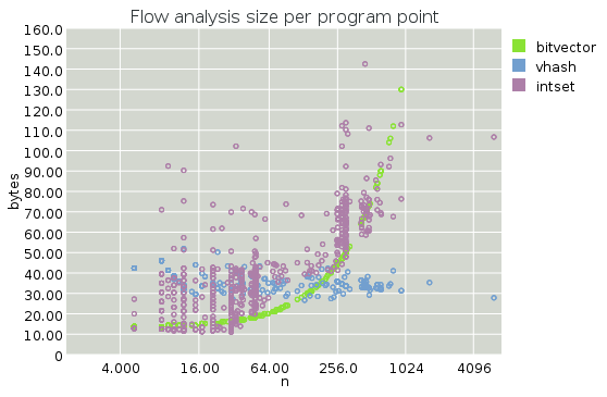
Note that the X axis is on a log scale.

The first thing that pops out at me from these graphs is that the per-label overhead vhash sizes are indeed constant. This is a somewhat surprising result for me; I thought that iterated convergence would make this overhead depend on the size of the program being compiled.

Secondly we see that the bitvector approach, while quadratic in overall program size, is still smaller until we get to about 1000 labels. It's hard to beat the constant factor for packed bitvectors! Note that I restricted the Y range, and the sizes for the bitvector approach are off the charts for N > 1024.

The intset size is, as we expected, asymptotically worse than vhashes, but overall not bad. It stays on the chart at least. Surprisingly, intsets are often better than vhashes for small functions, where we can avoid allocating branches at all -- note the "shelves" in the intset memory usage, at 32 and 256 entries, respectively, corresponding to the sizes that require additional levels in the tree. Things keep on rising with n, but sublinearly (again, recall that the X axis is on a log scale).

Next, a plot of how many nanoseconds it takes per label to solve the DFA equation above.

Here we see, as expected, intsets roundly beating vhashes for all n greater than about 200 or so, and show sublinear dependence on program size.

The good results for vhashes for the largest program are because the largest program in this file doesn't have any loops, and hardly any branching either. It's the best case for vhashes: all appends and no branches. Unfortunately, it's not the normal case.

It's not quite fair to compare intsets to bitvectors, as Guile's bitvectors are implemented in C and intsets are implemented in Scheme, which runs on a bytecode VM right now. But still, the results aren't bad, with intsets even managing to beat bitvectors for the biggest function. The gains there probably pay for the earlier losses.

This is a good result, considering that the goal was to reduce the space complexity of the algorithm. The 1-bit case is also the hardest case; when the state size grows, as in type inference, the gains of using structure-sharing trees grow accordingly.

conclusion

Let's wrap up this word-slog. A few things to note.

Before all this DFA work in Guile, I had very little appreciation of the dangers of N-squared complexity. I mean, sometimes I had to to think about it, but not often, expecially if your constant factors are low, or so I thought. But I got burned by it; hopefully the next time, if any, will be a long time coming.

I was happily, pleasantly surprised at the expressiveness and power of Bagwell/Clojure-style persistent data structures when applied to the kinds of problems that I work on. Space-sharing can make a fundamental difference to the characteristics of an algorithm, and Bagwell's data structures can do that well. Intsets simplified my implementations because I didn't have to reason much about space-sharing on my own -- finding the right shared tail for vhashes is, as I said, an unmitigated mess.

Finally I would close by saying that I was happy to fail in such interesting (to me) ways. It has been a pleasant investigation and I hope I have been able to convey some of the feeling of it. If you want to see what the resulting algorithm looks like in practice, see compute-truthy-expressions.

Until next time, happy hacking!